Linear Regression
Overview and Refresher
Week 2 Practice in Lab
Step 1: Set the working directory for reading in files.
setwd('/insert full path to your folder’) Remember, if you can’t get the setwd (set working directory) function to work, try ?setwd to get some additional help.
Step 2: Read csv file from on-line source.
You can read the data set from on-line as the cvs file in R
Ads <- read.csv("http://faculty.marshall.usc.edu/gareth-james/ISL/Advertising.csv")
#read.csv("/home/jsshingl1/data/Ads")
summary(Ads)

##        X                TV             radio          newspaper
##  Min.   :  1.00   Min.   :  0.70   Min.   : 0.000   Min.   :  0.30
##  1st Qu.: 50.75   1st Qu.: 74.38   1st Qu.: 9.975   1st Qu.: 12.75
##  Median :100.50   Median :149.75   Median :22.900   Median : 25.75
##  Mean   :100.50   Mean   :147.04   Mean   :23.264   Mean   : 30.55
##  3rd Qu.:150.25   3rd Qu.:218.82   3rd Qu.:36.525   3rd Qu.: 45.10
##  Max.   :200.00   Max.   :296.40   Max.   :49.600   Max.   :114.00
##      sales
##  Min.   : 1.60
##  1st Qu.:10.38
##  Median :12.90
##  Mean   :14.02
##  3rd Qu.:17.40
##  Max.   :27.00
Step 3a: Estimating the coefficients for simple linear regression
Now we will try to estimate the coefficients of the linear regression line. In order to estimate the coefficients we will use “lm” function. This function is already in the default R setting.
In Ads dataset, we have five variables: X, TV, radio, newspaper, and sales. X is a label of each data point. TV is a budget for TV ads. radio is a budget for ads in ratio. newspaper is a budget for ads in newspapers. They are all in thousands of dollars. We, here, want to ask the following question: Is there a relationship between advertising budget and sales? To answer this question we will try to fit the data with a simple linear regression model. First we will try to see any linear relation between sales and TV ads. Here sales as y variable, response and TV as x variable, explanatory.
lm.fit<-lm(sales~TV, data=Ads)
summary(lm.fit)

##
## Call:
## lm(formula = sales ~ TV, data = Ads)
##
## Residuals:
##     Min      1Q  Median      3Q     Max
## -8.3860 -1.9545 -0.1913  2.0671  7.2124
##
## Coefficients:
##             Estimate Std. Error t value Pr(>|t|)
## (Intercept) 7.032594   0.457843   15.36   <2e-16 ***
## TV          0.047537   0.002691   17.67   <2e-16 ***
## ---
## Signif. codes:  0 '***' 0.001 '**' 0.01 '*' 0.05 '.' 0.1 ' ' 1
##
## Residual standard error: 3.259 on 198 degrees of freedom
## Multiple R-squared:  0.6119, Adjusted R-squared:  0.6099
## F-statistic: 312.1 on 1 and 198 DF,  p-value: < 2.2e-16
If you want to print just estimates of coefficients…
lm.fit<-lm(sales~TV, data=Ads)
coef(lm.fit)

## (Intercept)          TV
##  7.03259355  0.04753664
If you want to print the confidence intervals for each estimate, type:
confint(lm.fit)

##                  2.5 %     97.5 %
## (Intercept) 6.12971927 7.93546783
## TV          0.04223072 0.05284256
Step 3b: Now let’s plot the regression line with the data points.
The sales are stored in the fourth column of the dataset “Ads” which is a two dimensional array.
head(Ads[,4])

## [1] 69.2 45.1 69.3 58.5 58.4 75.0

#or Ads$sales
Here Ads[,5] means the fifth column of the matrix “Ads”. If you want to access the fifth rows type Ads[5,] instead. Make sure the index starts from 1. NOT 0. In Python it starts 0. These numbers are set as a response variable.
TV is stored in the first column of the matrix “Ads”.
head(Ads$TV)

## [1] 230.1  44.5  17.2 151.5 180.8   8.7
These values are set as an explanatory variable.
In order to plot Ads$TV as y axis and Ads$sales as x axis using plot() function, type:
plot(Ads$TV,Ads$sales)

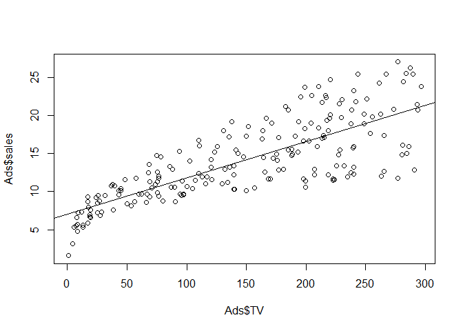
Then we want to add a regression line in the plot. You will use abline() function
lm.fit<-lm(sales~TV, data=Ads)
plot(Ads$TV,Ads$sales)
abline(lm.fit)
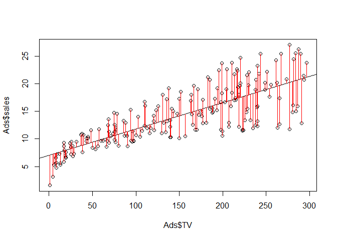
If you want to draw the residual lines as you have seen in the lecture you can type:
lm.fit<-lm(sales~TV, data=Ads)
plot(Ads$TV,Ads$sales)
abline(lm.fit)
pre <- predict(lm.fit)
segments(Ads$TV,Ads$sales, Ads$TV, pre, col="red")
Step 4: Estimating the coefficients for multiple linear regression
Now we will fit the data to multiple regression model. We will set TV, radio, and newspaper as explanatory variables, X1, X2, X3, and sales as a response variable, Y. To use lm() function for multiple linear regression, you have to set the model. To define we will do type “sales ~ TV+radio+newspaper”.
lm.fit<-lm(sales~TV+radio+newspaper, data=Ads)
summary(lm.fit)

##
## Call:
## lm(formula = sales ~ TV + radio + newspaper, data = Ads)
##
## Residuals:
##     Min      1Q  Median      3Q     Max
## -8.8277 -0.8908  0.2418  1.1893  2.8292
##
## Coefficients:
##              Estimate Std. Error t value Pr(>|t|)
## (Intercept)  2.938889   0.311908   9.422   <2e-16 ***
## TV           0.045765   0.001395  32.809   <2e-16 ***
## radio        0.188530   0.008611  21.893   <2e-16 ***
## newspaper   -0.001037   0.005871  -0.177     0.86
## ---
## Signif. codes:  0 '***' 0.001 '**' 0.01 '*' 0.05 '.' 0.1 ' ' 1
##
## Residual standard error: 1.686 on 196 degrees of freedom
## Multiple R-squared:  0.8972, Adjusted R-squared:  0.8956
## F-statistic: 570.3 on 3 and 196 DF,  p-value: < 2.2e-16
For a short cut you can do
lm.fit<-lm(sales~., data=Ads)
summary(lm.fit)

##
## Call:
## lm(formula = sales ~ ., data = Ads)
##
## Residuals:
##     Min      1Q  Median      3Q     Max
## -8.8105 -0.9008  0.2641  1.1783  2.8336
##
## Coefficients:
##               Estimate Std. Error t value Pr(>|t|)
## (Intercept)  3.0052094  0.3942082   7.623 1.06e-12 ***
## X           -0.0005798  0.0020992  -0.276    0.783
## TV           0.0457759  0.0013988  32.725  < 2e-16 ***
## radio        0.1883832  0.0086480  21.784  < 2e-16 ***
## newspaper   -0.0012433  0.0059319  -0.210    0.834
## ---
## Signif. codes:  0 '***' 0.001 '**' 0.01 '*' 0.05 '.' 0.1 ' ' 1
##
## Residual standard error: 1.689 on 195 degrees of freedom
## Multiple R-squared:  0.8973, Adjusted R-squared:  0.8951
## F-statistic: 425.7 on 4 and 195 DF,  p-value: < 2.2e-16
What do you think the difference between “lm.fit<-lm(sales~TV+radio+newspaper, data=Ads)” and “lm.fit<-lm(sales~., data=Ads)”? In lm() function, if we type as “sales~.” then we are assigning ALL variables except sales as explanatory variables.
What is your answers to the following questions?
Is at least one of the predictors X1, X2, . . . , Xp useful in predicting the response?
Do all the predictors help to explain Y, or is only a subset of the predictors useful?
How well does the model fit the data?
What does the coefficient for the newspaper variable suggest?
Before moving on, perform the following three actions to save your work and prepare for the practical application: Save your workspace as “LectureExampleData1.RData” (By typing save.image(“LectureExampleData1.RData”) function)